pacman::p_load(stargazer, # Reporte
sjPlot, sjmisc, # reporte y gráficos
sjlabelled,
corrplot, # grafico correlaciones
xtable, # Reporte
Hmisc, # varias funciones
psych, # fa y principal factors
psy, # scree plot function
nFactors, # parallel
GPArotation) # rotaciónAnálisis Factorial Exploratorio
Librerías y Datos
Librerías
Datos
Lectura de datos
data <- read.csv("input/data/efa_asignaturas.csv")- Muestra de 300 alumnos a los que se le pregunta por su asignatura favorita en una escala de 1 (no me agrada) a 5 (me agrada)
Exploración de datos
summary(data) BIO GEO CHEM ALG CALC
Min. :1.000 Min. :1.00 Min. :1.000 Min. :1.00 Min. :1.000
1st Qu.:1.000 1st Qu.:1.00 1st Qu.:1.000 1st Qu.:2.00 1st Qu.:2.000
Median :2.000 Median :2.00 Median :2.000 Median :3.00 Median :3.000
Mean :2.353 Mean :2.17 Mean :2.237 Mean :3.05 Mean :3.063
3rd Qu.:3.000 3rd Qu.:3.00 3rd Qu.:3.000 3rd Qu.:4.00 3rd Qu.:4.000
Max. :5.000 Max. :5.00 Max. :5.000 Max. :5.00 Max. :5.000
STAT
Min. :1.000
1st Qu.:2.000
Median :3.000
Mean :2.937
3rd Qu.:4.000
Max. :5.000 names(data)[1] "BIO" "GEO" "CHEM" "ALG" "CALC" "STAT"dim(data) # filas columnas[1] 300 6nrow(na.omit(data)) # número de casos con datos completos[1] 300Descriptivos
stargazer(data, type = "text") # para visualizar en consola
====================================
Statistic  N  Mean  St. Dev. Min Max
------------------------------------
BIO       300 2.353  1.228    1   5
GEO       300 2.170  1.230    1   5
CHEM      300 2.237  1.273    1   5
ALG       300 3.050  1.174    1   5
CALC      300 3.063  1.127    1   5
STAT      300 2.937  1.259    1   5
------------------------------------stargazer(data, type = "html") # a html| Statistic | N | Mean | St. Dev. | Min | Max |
| BIO | 300 | 2.353 | 1.228 | 1 | 5 |
| GEO | 300 | 2.170 | 1.230 | 1 | 5 |
| CHEM | 300 | 2.237 | 1.273 | 1 | 5 |
| ALG | 300 | 3.050 | 1.174 | 1 | 5 |
| CALC | 300 | 3.063 | 1.127 | 1 | 5 |
| STAT | 300 | 2.937 | 1.259 | 1 | 5 |
Gráfico barras apiladas
#sjplot(data$BIO, "frq") # no muy buena descripción ...

names(data)
[1] "BIO" "GEO" "CHEM" "ALG" "CALC" "STAT"plot_stackfrq(data)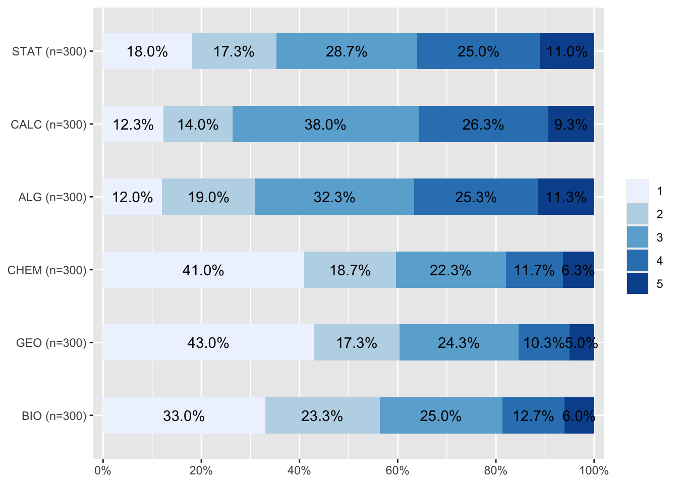
Gráfico final
#label values

data <- data %>%  set_labels (., labels=c("No le agrada"=1,
  "Le agrada"=5))

plot_stackfrq(data, sort.frq = "last.desc", geom.colors = "OrRd") #+ theme(legend.position="bottom")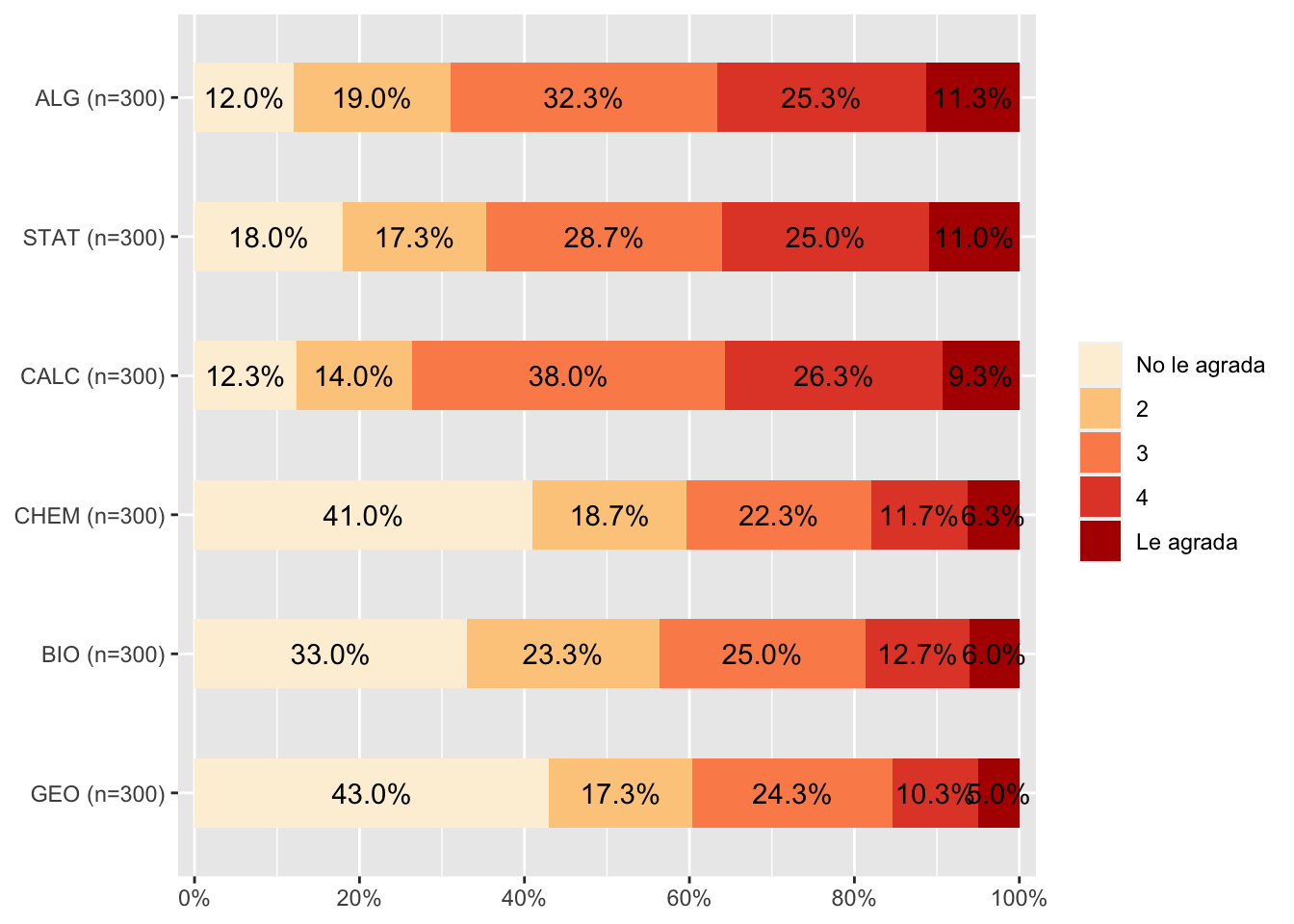
Analisis de matriz de correlaciones
Matriz
corMat  <- cor(data)  # estimar matriz pearson
options(digits=2)
corMat # muestra matriz
BIO GEO CHEM ALG CALC STAT
BIO 1.00 0.68 0.747 0.115 0.21 0.20
GEO 0.68 1.00 0.681 0.135 0.20 0.23
CHEM 0.75 0.68 1.000 0.084 0.14 0.17
ALG 0.12 0.14 0.084 1.000 0.77 0.41
CALC 0.21 0.20 0.136 0.771 1.00 0.51
STAT 0.20 0.23 0.166 0.409 0.51 1.00Reporte tabla
tab_corr(data, triangle = "lower")| BIO | GEO | CHEM | ALG | CALC | STAT | |
| BIO | ||||||
| GEO | 0.682*** | |||||
| CHEM | 0.747*** | 0.681*** | ||||
| ALG | 0.115* | 0.135* | 0.084 | |||
| CALC | 0.213*** | 0.205*** | 0.136* | 0.771*** | ||
| STAT | 0.203*** | 0.232*** | 0.166** | 0.409*** | 0.507*** | |
| Computed correlation used pearson-method with listwise-deletion. | ||||||
Reporte gráfico con corrplot
M=cor(data) # matriz simple de correlaciones de los datos
corrplot(M, type="lower") # lower x bajo diagonal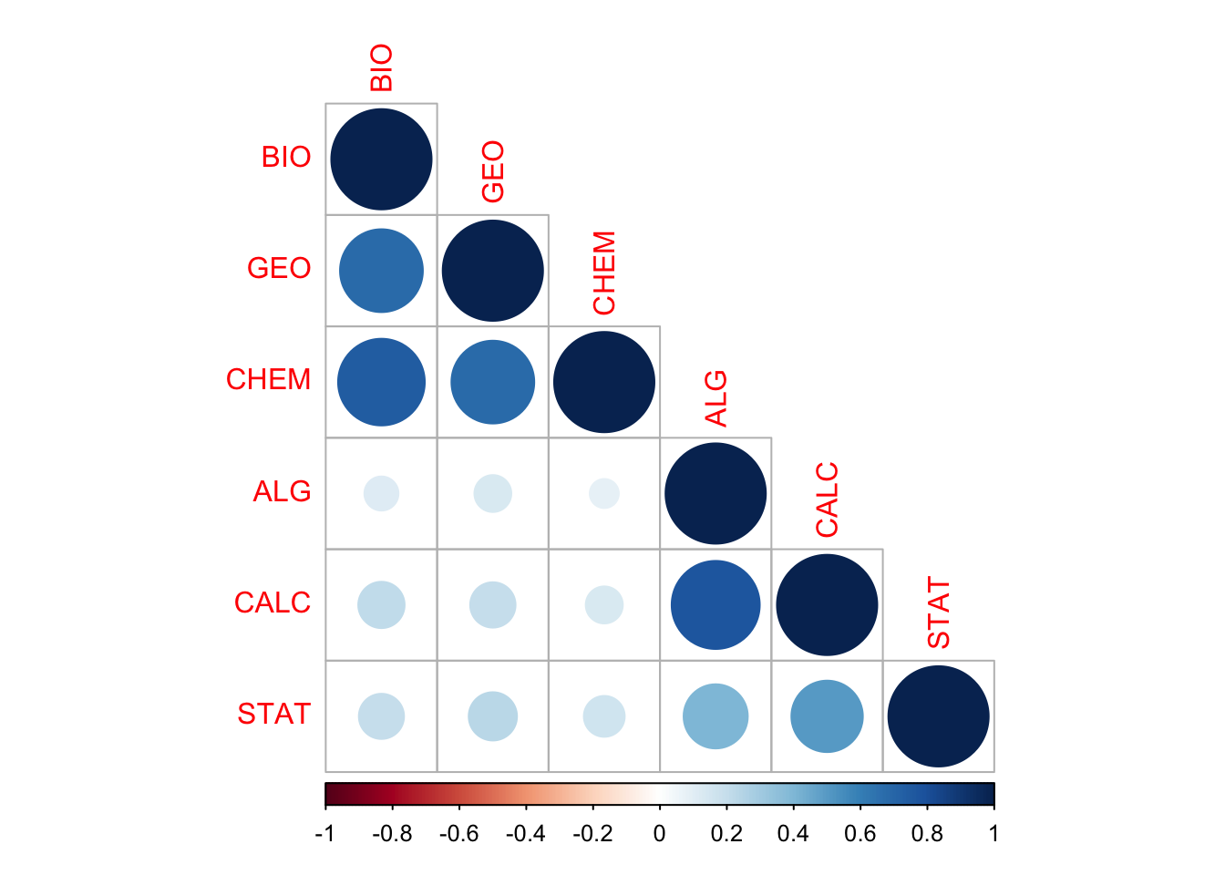
Otra opción
corrplot(M, type="lower",
      order="AOE", cl.pos="b", tl.pos="d") #agrega nombres en diag.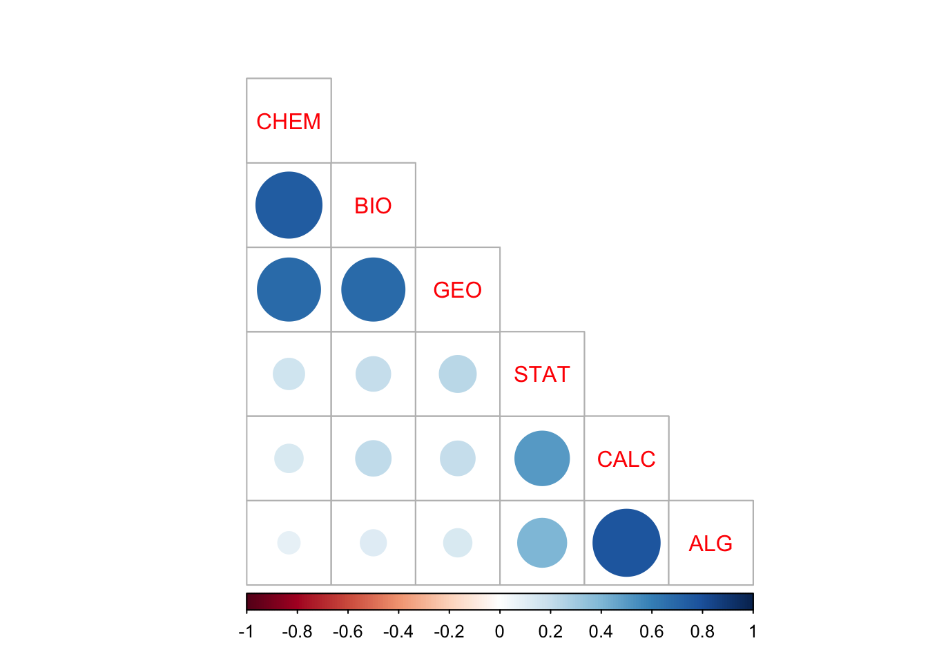
Análisis factorial
¿Qué se puede deducir de la matriz de correlaciones en relación a la estructura subyacente en términos de variables latentes? Vemos dos grupos de indicadores asociados entre sí, y no asociados con el otro grupo. Por un lado, el grupo de chem, bio y geo, y por otro el de stat, calc y alg.
Adecuación de matriz para análisis factorial
KMO(corMat)Kaiser-Meyer-Olkin factor adequacy
Call: KMO(r = corMat)
Overall MSA = 0.7
MSA for each item =
BIO GEO CHEM ALG CALC STAT
0.73 0.81 0.72 0.60 0.60 0.84 cortest.bartlett(corMat, n = 300)$chisq
[1] 849
$p.value
[1] 2.6e-171
$df
[1] 15Seleccion de numero de factores
Graficos
scree.plot(data)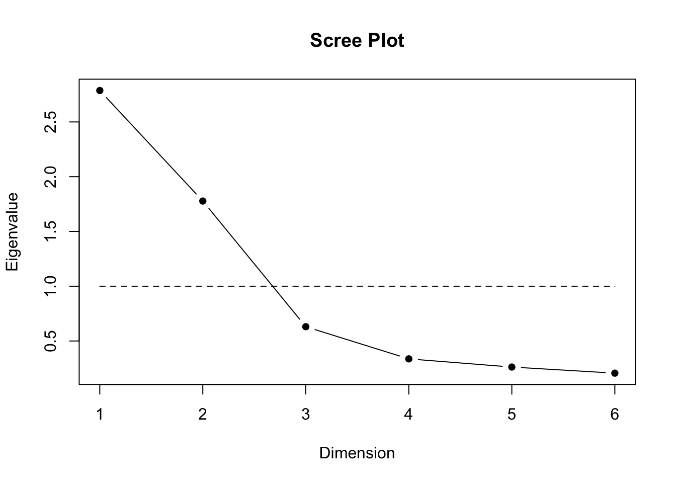
fa.parallel(corMat, n.obs=300)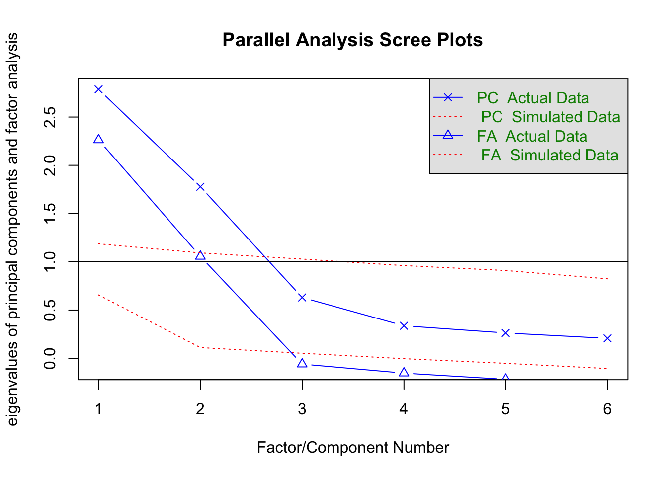
Parallel analysis suggests that the number of factors = 2 and the number of components = 2 library(nFactors)
ev <- eigen(corMat) # get eigenvalues
ap <- parallel(subject=300,var=6,
rep=100,cent=.05)
nS <- nScree(x=ev$values, aparallel=ap$eigen$qevpea)
plotnScree(nS)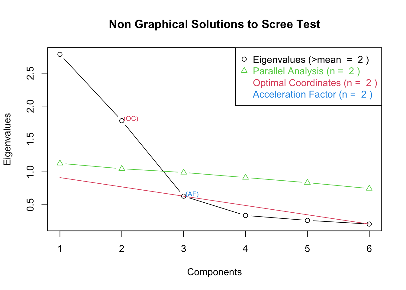
Factor de aceleración: solución numérica que muestra el punto que presenta el mayor cambio de pendiente
Optimal coordinates: muestra el primer eigenvalue que puede ser mejor “extrapolado” desde el eigenvalue previo (“optimal coordinates are the extrapolated coordinates of the previous eigenvalue that allow the observed eigenvalue to go beyond this extrapolation” (http://www.inside-r.org/packages/cran/nFactors/docs/nScree)
Extracción
Ejes principales
fac_pa <- fa(r = data, nfactors = 2, fm= "pa")
#summary(fac_pa)
fac_pa
Factor Analysis using method = pa
Call: fa(r = data, nfactors = 2, fm = "pa")
Standardized loadings (pattern matrix) based upon correlation matrix
PA1 PA2 h2 u2 com
BIO 0.86 0.02 0.75 0.255 1.0
GEO 0.78 0.05 0.63 0.369 1.0
CHEM 0.87 -0.05 0.75 0.253 1.0
ALG -0.04 0.81 0.65 0.354 1.0
CALC 0.01 0.96 0.92 0.081 1.0
STAT 0.13 0.50 0.29 0.709 1.1
PA1 PA2
SS loadings 2.14 1.84
Proportion Var 0.36 0.31
Cumulative Var 0.36 0.66
Proportion Explained 0.54 0.46
Cumulative Proportion 0.54 1.00
With factor correlations of
PA1 PA2
PA1 1.00 0.21
PA2 0.21 1.00
Mean item complexity = 1
Test of the hypothesis that 2 factors are sufficient.
df null model = 15 with the objective function = 2.9 with Chi Square = 849
df of the model are 4 and the objective function was 0.01
The root mean square of the residuals (RMSR) is 0.01
The df corrected root mean square of the residuals is 0.02
The harmonic n.obs is 300 with the empirical chi square 0.78 with prob < 0.94
The total n.obs was 300 with Likelihood Chi Square = 3.3 with prob < 0.51
Tucker Lewis Index of factoring reliability = 1
RMSEA index = 0 and the 90 % confidence intervals are 0 0.08
BIC = -20
Fit based upon off diagonal values = 1
Measures of factor score adequacy
PA1 PA2
Correlation of (regression) scores with factors 0.94 0.96
Multiple R square of scores with factors 0.88 0.93
Minimum correlation of possible factor scores 0.77 0.86Maximum likelihood
fac_ml <- fa(r = data, nfactors = 2, fm= "ml")
summary(fac_ml)
Plot de cargas factoriales ml
factor.plot(fac_ml, labels=rownames(fac_ml$loadings))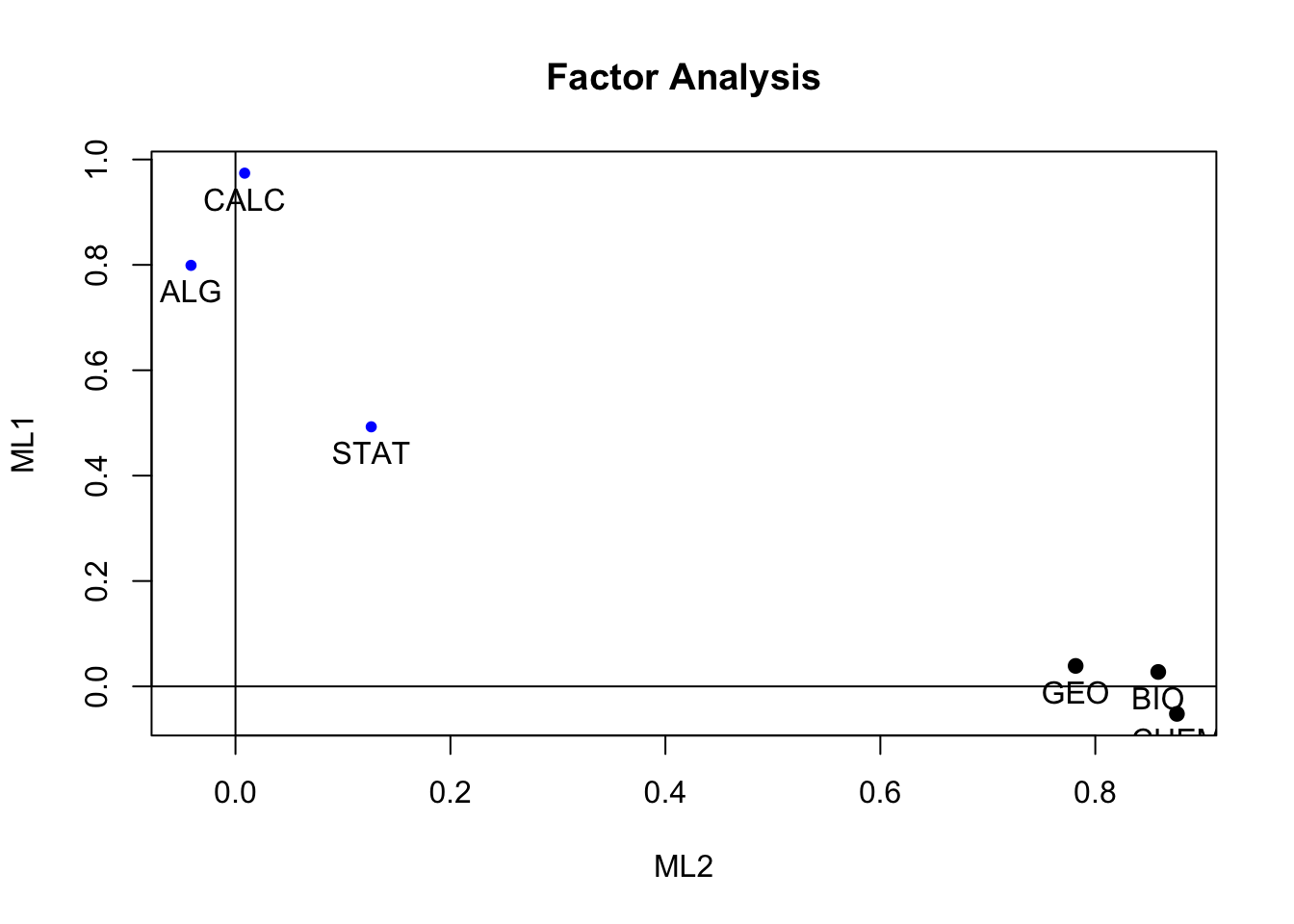
Obtención de Puntajes factoriales
Los puntajes factoriales son vectores/variables que representan al factor latente como una variable observada y que por lo tanto suma una columna a la base de datos por cada factor extraído. Como la variable latente no tiene métrica, se le otorga una con media 0 y varianza 1. Los puntajes son una especie de índice pero donde la constribución de cada indicador al índice se encuentra ponderada por su carga factorial (su contribución a la variable latente común o factor).
fac_ml <- fa(r = data, nfactors = 2, fm= "ml", scores="regression")
data2=data
data3 <- cbind(data2, fac_ml$scores)
head(data3)
BIO GEO CHEM ALG CALC STAT ML2 ML1
1 1 1 1 1 1 1 -1.110 -1.84
2 4 4 3 4 4 4 1.153 0.85
3 2 1 3 4 1 1 -0.188 -1.61
4 2 3 2 4 4 3 -0.013 0.82
5 3 1 2 2 3 4 -0.070 -0.11
6 1 1 1 4 4 4 -1.022 0.84Rotación
Varimax (ortogonal)
fac_ml_var <- fa(r = data, nfactors = 2, fm= "ml", rotate="varimax") # ortogonal
fac_ml_var
Factor Analysis using method = ml
Call: fa(r = data, nfactors = 2, rotate = "varimax", fm = "ml")
Standardized loadings (pattern matrix) based upon correlation matrix
ML2 ML1 h2 u2 com
BIO 0.85 0.13 0.75 0.252 1.0
GEO 0.78 0.13 0.63 0.375 1.1
CHEM 0.86 0.06 0.75 0.249 1.0
ALG 0.03 0.79 0.63 0.374 1.0
CALC 0.10 0.97 0.95 0.048 1.0
STAT 0.17 0.51 0.29 0.715 1.2
ML2 ML1
SS loadings 2.12 1.86
Proportion Var 0.35 0.31
Cumulative Var 0.35 0.66
Proportion Explained 0.53 0.47
Cumulative Proportion 0.53 1.00
Mean item complexity = 1.1
Test of the hypothesis that 2 factors are sufficient.
df null model = 15 with the objective function = 2.9 with Chi Square = 849
df of the model are 4 and the objective function was 0.01
The root mean square of the residuals (RMSR) is 0.01
The df corrected root mean square of the residuals is 0.02
The harmonic n.obs is 300 with the empirical chi square 0.97 with prob < 0.91
The total n.obs was 300 with Likelihood Chi Square = 2.9 with prob < 0.57
Tucker Lewis Index of factoring reliability = 1
RMSEA index = 0 and the 90 % confidence intervals are 0 0.076
BIC = -20
Fit based upon off diagonal values = 1
Measures of factor score adequacy
ML2 ML1
Correlation of (regression) scores with factors 0.94 0.98
Multiple R square of scores with factors 0.88 0.95
Minimum correlation of possible factor scores 0.76 0.91Promax (oblicua)
fac_ml_pro <- fa(r = data, nfactors = 2, fm= "ml", rotate="promax")
fac_ml_pro
Factor Analysis using method = ml
Call: fa(r = data, nfactors = 2, rotate = "promax", fm = "ml")
Standardized loadings (pattern matrix) based upon correlation matrix
ML2 ML1 h2 u2 com
BIO 0.86 0.02 0.75 0.252 1.0
GEO 0.78 0.03 0.63 0.375 1.0
CHEM 0.88 -0.06 0.75 0.249 1.0
ALG -0.09 0.81 0.63 0.374 1.0
CALC -0.05 0.99 0.95 0.048 1.0
STAT 0.10 0.50 0.29 0.715 1.1
ML2 ML1
SS loadings 2.12 1.86
Proportion Var 0.35 0.31
Cumulative Var 0.35 0.66
Proportion Explained 0.53 0.47
Cumulative Proportion 0.53 1.00
With factor correlations of
ML2 ML1
ML2 1.00 0.28
ML1 0.28 1.00
Mean item complexity = 1
Test of the hypothesis that 2 factors are sufficient.
df null model = 15 with the objective function = 2.9 with Chi Square = 849
df of the model are 4 and the objective function was 0.01
The root mean square of the residuals (RMSR) is 0.01
The df corrected root mean square of the residuals is 0.02
The harmonic n.obs is 300 with the empirical chi square 0.97 with prob < 0.91
The total n.obs was 300 with Likelihood Chi Square = 2.9 with prob < 0.57
Tucker Lewis Index of factoring reliability = 1
RMSEA index = 0 and the 90 % confidence intervals are 0 0.076
BIC = -20
Fit based upon off diagonal values = 1
Measures of factor score adequacy
ML2 ML1
Correlation of (regression) scores with factors 0.94 0.98
Multiple R square of scores with factors 0.89 0.96
Minimum correlation of possible factor scores 0.77 0.91Reporte: Tabla análisis factorial
A html via sjPlot
tab_fa(data, rotation = "varimax",show.comm = TRUE, title = "Análisis factorial asignaturas")Parallel analysis suggests that the number of factors = 2 and the number of components = NA | Factor 1 | Factor 2 | Communality | |
| BIO | 0.85 | 0.13 | 0.75 |
| GEO | 0.78 | 0.13 | 0.63 |
| CHEM | 0.86 | 0.06 | 0.75 |
| ALG | 0.03 | 0.79 | 0.63 |
| CALC | 0.10 | 0.97 | 0.95 |
| STAT | 0.17 | 0.51 | 0.29 |
| Total Communalities | 3.99 | ||
| Cronbach's α | 0.88 | 0.79 | |
Código
El código de esta página se encuentra disponible en el repositorio del curso en Github